


Don’t be Fooled by QE Taper Talk
Interest-Rates / Quantitative Easing May 22, 2014 - 05:05 PM GMTBy: Steve_H_Hanke

 Since last June, most thought the U.S. Federal Reserve’s so-called taper was just around the corner. Well, the Fed’s large-scale asset purchasers did finally begin to take action, but they did so later than most anticipated. It now appears that the door will close on the Fed’s massive asset purchase program late this year. With this in mind, talk has turned to another aspect of the taper – just when will the Fed start to increase the federal funds interest rate? It probably won’t be anytime soon. Yes, the massive distortions created by the Fed’s interest rate manipulations (read: carry trade, among others) will be with us for longer than most anticipate. Why?
The U.S. is still in the midst of the Great Recession. Yes, there have been recent encouraging economic reports. But, the U.S. economy remains weak and vulnerable. Aggregate demand (measured by final sales to domestic purchasers) tells the tale (see the accompanying chart). The annual trend rate of growth in nominal aggregate demand has been 4.95% since 1987. At the depth of the Great Recession, that metric plunged to a negative annual rate of more than -4.0%. However, aggregate demand bounced back. Indeed, it almost reached the trend rate of growth in late 2011. But, since then, it has slumped to its current 2.86% annual rate. Remarkably, this is very close to the rate of growth in aggregate demand that prevailed during the recession of 1990-91 – the recession that probably cost President George H.W. Bush his bid for a second term.

Just why is the U.S. nominal aggregate demand so weak? It’s all about money. Money dominates. Before we jump to the current status of the money supply, we must ask, what’s the correct measure for the money supply?
To answer that question, we flash back to 1979, when Paul Volcker took the reins of the Federal Reserve System. The state of the economy was dreadful, with double-digit annual inflation running at 13.3%.
Chairman Volcker realized that money matters, and it didn’t take him long to make his move. On Saturday, 6 October 1979, he stunned the world with an unanticipated announcement. He proclaimed that he was going to put measures of the money supply on the Fed’s dashboard. For him, it was obvious that, to restore the U.S. economy to good health, inflation would have to be wrung out of the economy. And to kill inflation, the money supply would have to be controlled.
Chairman Volcker achieved his goal. By 1982, the annual rate of inflation had dropped to 3.8% – a great accomplishment. The problem was that the Volcker inflation squeeze brought with it a relatively short recession (less than a year) that started in January 1980, and another, more severe slump that began shortly thereafter and ended in November 1982.
Chairman Volcker’s problem was that the monetary speedometer installed on his dashboard was defective. Each measure of the money supply (M1, M2, M3 and so forth) was shown on a separate gauge, with the various measures being calculated by a simple summation of their components. The components of each measure were given the same weight, implying that all of the components possessed the same degree of moneyness – usefulness in immediate transactions where money is exchanged between buyer and seller.
As shown in the accompanying chart, the Fed thought that the double-digit fed funds rates it was serving up were allowing it to tap on the money-supply brakes with just the right amount of pressure. In fact, if the money supply had been measured correctly by a Divisia metric, Chairman Volcker would have realized that the Fed was slamming on the brakes from 1978 until early 1982. The Fed was imposing a monetary policy that was much tighter than it thought.

Why is the Divisia metric the superior money supply measure, and why did it diverge so sharply from the Fed’s conventional measure (M2)? Money takes the form of various types of financial assets that are used for transaction purposes and as a store of value. Money created by a monetary authority (notes, coins, and banks’ deposits at the monetary authority) represents the underlying monetary base of an economy. This state money, or high-powered money, is imbued with the most moneyness of the various types of financial assets that are called money. The monetary base is ready to use in transactions in which goods and services are exchanged for “money.”
In addition to the assets that make up base money, there are many others that possess varying degrees of moneyness – a characteristic which can be measured by the ease of and the opportunity costs associated with exchanging them for base money. These other assets are, in varying degrees, substitutes for money. That is why they should not receive the same weights when they are summed to obtain a broad money supply measure. Instead, those assets that are the closest substitutes for base money should receive higher weights than those that possess a lower degree of moneyness.
Now, let’s come back to the huge divergences between the standard simple-sum measures of M2 that Chairman Volcker was observing and the true Divisia M2 measure. As the Fed pushed the fed funds rate up, the opportunity cost of holding cash increased. In consequence, retail money market funds and time deposits, for example, became relatively more attractive and received a lower weight when measured by a Divisia metric. Faced with a higher interest rate, people had a much stronger incentive to avoid “large” cash and checking account balances. As the fed funds rate went up, the divergence between the simple-sum and Divisia M2 measures became greater and greater.
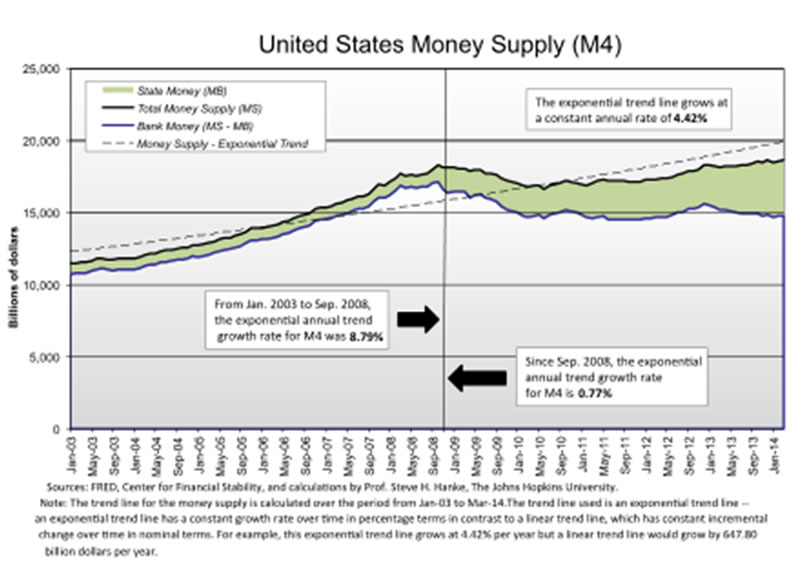
When available, Divisia measures are the “best” measures of the money supply. But, how many classes of financial assets that possess moneyness should be added together to determine the money supply? This is a case in which the phrase “the more the merrier” applies. When it comes to money, the broadest measure is the best. In the U.S., we are fortunate to have Divisia M4 available from the Center for Financial Stability in New York. The data for Divisia M4 in the accompanying chart show why the U.S. nominal aggregate demand and overall economy have followed the course that they have, and why the U.S. is still in the grip of the Great Recession. After all, even now, the annual Divisia M4 growth rate is an anemic 2.6%.
But why has the Divisia M4 growth rate been so slow since the collapse of Lehman Brothers? It’s not because the Fed has taken its foot off the state money accelerator. The anemic growth of the total money supply, broadly measured, results from an outright drop in the quantity of bank money in the economy since the Lehman collapse. Since bank money accounts for 80% of the Divisia M4 measure (making it the big elephant in the room), its decrease has dragged down the overall money supply growth rate (see the accompanying chart).
But why? Tougher bank supervision, stricter prudential bank regulations, and higher bank capital requirements provide the answer. Don’t look for any of these three procyclical squeezes on bank money to be released anytime soon.
In consequence, the Fed will probably be forced to keep federal funds at the zero bound much longer than most think – perhaps well into 2016.
By Steve H. Hanke
www.cato.org/people/hanke.html
Twitter: @Steve_Hanke
Steve H. Hanke is a Professor of Applied Economics and Co-Director of the Institute for Applied Economics, Global Health, and the Study of Business Enterprise at The Johns Hopkins University in Baltimore. Prof. Hanke is also a Senior Fellow at the Cato Institute in Washington, D.C.; a Distinguished Professor at the Universitas Pelita Harapan in Jakarta, Indonesia; a Senior Advisor at the Renmin University of China’s International Monetary Research Institute in Beijing; a Special Counselor to the Center for Financial Stability in New York; a member of the National Bank of Kuwait’s International Advisory Board (chaired by Sir John Major); a member of the Financial Advisory Council of the United Arab Emirates; and a contributing editor at Globe Asia Magazine.
Copyright © 2014 Steve H. Hanke - All Rights Reserved
Disclaimer: The above is a matter of opinion provided for general information purposes only and is not intended as investment advice. Information and analysis above are derived from sources and utilising methods believed to be reliable, but we cannot accept responsibility for any losses you may incur as a result of this analysis. Individuals should consult with their personal financial advisors.
Steve H. Hanke Archive |
© 2005-2022 http://www.MarketOracle.co.uk - The Market Oracle is a FREE Daily Financial Markets Analysis & Forecasting online publication.