Why Hasn't the U.S. Economic Stimulus Been More Stimulative?
Economics / Economic Stimulus Aug 23, 2010 - 06:40 PM GMTBy: Paul_L_Kasriel
 Talk of the economy slipping back into a recession is rampant. The American Recovery and Reconstruction Act (ARRA) of 2009, aka the stimulus package of approximately $790 billion, was, as its title suggests, supposed to put the economy firmly into a recovery trajectory. But as Obama administration economic guru has said, the economy is having trouble reaching recession-escape velocity. Why hasn't the 2009 stimulus package been more stimulative?
 For starters, of course, the federal government has been slow in disbursing funds - a genuine case of man bites dog. According to ProPublica.com, as of August 9, $65 billion of the $288 billion of tax cuts, or 23% of the tax cuts, is yet at the disposal of households and businesses. And $230 billion of the $502 billion, or 46% of the allocated spending, still is waiting to be spent. So there still is about 37% of ARRA sitting in the disbursement pipeline.
But I believe that there is a more important reason why ARRA has not been more stimulative in chumming up nominal aggregate demand. I believe that for fiscal policy to stimulate aggregate demand, it needs bank financing. Otherwise, fiscal policy mostly just re-allocates total aggregate demand toward government spending and away from private spending. Let's assume that the federal government increases its spending, financing this via the issuance of additional debt. And let's further assume that this debt is purchased by the nonbank public, including foreign entities. Now, I am going to make a simplifying assumption here by stipulating that the nonbank public cuts back on its current spending, i.e., increases its saving, in order to buy this additional government debt. Under this assumption, total spending in the economy would not increase as a result of the federal government's stimulus program. Rather, private sector current spending would fall by the same amount as government spending increased. An exception to this would be if the nonbank public was willing to rundown its money holdings in order to purchase the increased government debt rather than cut back on current spending. In this exceptional case, total spending could increase. This would be an example of what is referred to an increase in the velocity of money.
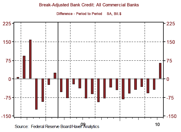
In contrast to the nonbank public purchasing the new government debt, if the banking system were to purchase the increase in government debt issued to finance the increase in government spending, then no nonbank entity would have to cut back on its current spending as the government increased its spending. In this case, the fiscal stimulus would stimulate aggregate demand. Government spending would increase without a corresponding decrease in private spending. It is not necessary that the banking system purchase government securities for the fiscal stimulus to stimulate. All that is required is that the banking system increases the total of its holdings of loans and investments by the amount of the increase in government debt. Chart 1 shows that in only one month, July 2010, since the ARRA legislation was signed into law in February 2009 has total bank credit increased. So, if my hypothesis is correct about the relative impotence of fiscal stimulus without corresponding "stimulus" from the banking system, we would not expect ARRA to have had much impact on nominal aggregate demand.
Chart 1

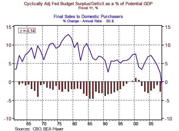
How does fiscal stimulus correlate with growth in nominal aggregate in the U.S.? Not all that well. Plotted in Chart 2 are the Congressional Budget Office's estimates of the cyclically-adjusted federal budget surpluses (+) and deficits (-) as a percent of potential GDP as well as the year-to-year percent change in nominal final sales to domestic purchasers - the aggregate demand concept most likely to be affected by fiscal stimulus. The reason for using the cyclically-adjusted budget surplus/deficit is to remove the normal cyclical variations in outlays (unemployment insurance benefit payments, etc) and normal cyclical variations in revenues (corporate tax payments, etc.). The correlation information between the cyclically-adjusted federal budget surplus/deficit and the percent change in nominal final sales to domestic purchasers is shown in the box in the top left-hand corner of Chart 2. A priori, we would expect a negative correlation between the behavior of the cyclically-adjusted budget surplus/deficit and the change in nominal aggregate demand. That is, the larger the deficit (a negative number), the larger the percentage increase in nominal aggregate demand growth. And this is just what is indicated by the minus sign in front of the 0.14 in the box. But the "0.14", the correlation coefficient, itself, is problematic for those advocating fiscal stimulus to reboot the economy. The highest possible reading on the correlation coefficient is 1.00, meaning that the two series are perfectly correlated. With the correlation coefficient at only 0.14, the implication is that the cyclically-adjusted surplus/deficit is only weakly correlated. But at least the sign is right!
Chart 2

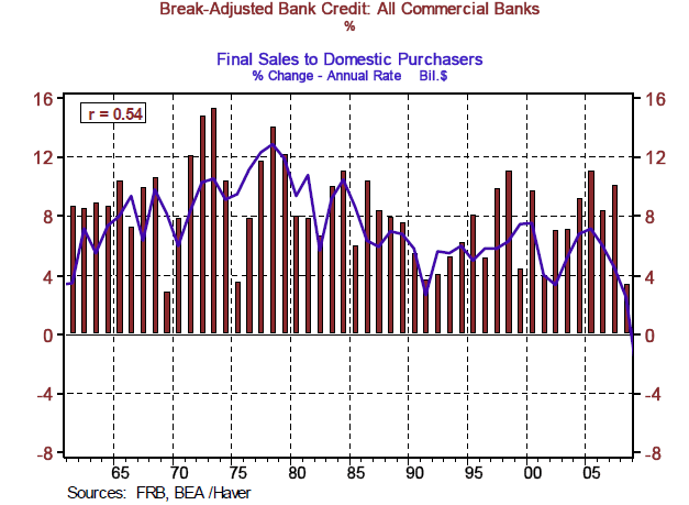
Chart 3 shows the relationship between the percent change in bank credit (loans and securities on the books of the banking system) and the percent change in nominal final sales to domestic purchasers. A priori, we would expect a positive correlation between the two. And the lack of a minus sign in front of the 0.54 correlation coefficient in the little box in the top left-hand corner of Chart 3 confirms this positive correlation. Notice that the magnitude of the correlation coefficient between bank credit and aggregate demand is much higher than that between the cyclically-adjusted surplus/deficit and aggregate demand.
Chart 3

In order to test for the separate effects on nominal aggregate demand growth of the cyclically-adjusted surplus/deficit and bank credit growth, we have to estimate an ordinary least-squares regression. When we estimate this regression with both explanatory variables included, we are, in effect, asking the following two questions: (1) "What is the effect on nominal aggregate demand growth when the cyclically-adjusted budget surplus/deficit changes, holding constant the rate of growth in bank credit?" and (2) "What is the effect on nominal aggregate demand growth when the growth in bank credit changes, holding constant the cyclically-adjusted budget deficit/surplus?"
But first let's run a regression with only the cyclically-adjusted budget surplus/deficit as the explanatory variable along with a constant, "c," term. This is shown in Table 1. It would be an understatement to say that the results of this regression would imply the impotency of fiscal policy to stimulate nominal aggregate demand growth. About the best you can say about this regression in terms of the effectiveness of fiscal policy to stimulate nominal aggregate demand growth is that the coefficient has the correct sign in front of it, a minus sign. But the magnitude of the t-statistic, at 0.916 (rounded) suggests the coefficient, or the effect of the cyclically-adjusted deficit as a percent of potential GDP, has a high probability of being zero, nada. Generally, a t-statistic value of 2.00 implies that there is a 95% probability that the value of the coefficient associated with the explanatory variable is different from zero. A minus sign in front of the adjusted R-squared coefficient is never encouraging, along with miniscule size of the coefficient (0.00 rounded, out of a possible maximum of 1.00). In other words, the cyclically-adjusted budget surplus/deficit as a percent of potential GDP appears to explain none of the movements in the growth of nominal final sales of domestic purchases.
Table 1
| Dependent Variable: Growth in Final Sales to Dom. Purchasers | ||||
| Method: Least Squares | ||||
| Sample: 1962 2008 | ||||
| Included observations: 47 | ||||
| Variable | Coefficient | Std. Error | t-Statistic | Prob. |
| Cyclically-Adjusted Deficit as a % of GDP | -0.260221 | 0.284032 | -0.916167 | 0.3645 |
| C | 6.850905 | 0.688854 | 9.945363 | 0.0000 |
| R-squared | 0.018311 | Mean dependent var | 7.388511 | |
| Adjusted R-squared | -0.003504 | S.D. dependent var | 2.469297 | |
| S.E. of regression | 2.473620 | |||
| Sum squared resid | 275.3457 | |||
| Log likelihood | -108.2353 | |||
| F-statistic | 0.839363 | Durbin-Watson stat | 0.551483 | |
| Prob(F-statistic) | 0.364463 | |||
Now let's run another regression, but this time using only bank credit growth as the explanatory variable along with a constant term. The results of this regression are shown in Table 2. The coefficient on growth in bank credit has the correct sign, positive. The t-statistic value of 4.429 (rounded) indicates that there is more than a 99% probability that the coefficient on bank credit growth is not zero. That is, there is a high probability that bank credit growth affects growth in nominal aggregate demand. The adjusted R-squared coefficient of 0.29 (rounded) is nothing to write home about, but at least is does suggest that growth in bank credit and a constant term do explain some of the variation in the growth of nominal final sales of domestic purchases.
Table 2
| Dependent Variable: Growth in Final Sales to Dom. Purchasers | ||||
| Method: Least Squares | ||||
| Sample: 1962 2008 | ||||
| Included observations: 47 | ||||
| Variable | Coefficient | Std. Error | t-Statistic | Prob. |
| Growth in Bank Credit | 0.454461 | 0.102609 | 4.429047 | 0.0001 |
| C | 3.612617 | 0.905076 | 3.991508 | 0.0002 |
| R-squared | 0.303583 | Mean dependent var | 7.388511 | |
| Adjusted R-squared | 0.288107 | S.D. dependent var | 2.469297 | |
| S.E. of regression | 2.083438 | |||
| Sum squared resid | 195.3322 | |||
| Log likelihood | -100.1671 | |||
| F-statistic | 19.61645 | Durbin-Watson stat | 0.987070 | |
| Prob(F-statistic) | 0.000060 | |||
Now it is time to run the regression with both the cyclically-adjusted budget surplus/deficit as a percent of potential GDP and bank credit growth as explanatory variables, along, of course, with a constant term. The results of this regression are in Table 3. Not surprisingly, the addition of the cyclically-adjusted budget surplus/deficit as a percent of potential GDP adds nothing to the explanation of the variation in the growth of nominal final sales to domestic purchasers as evidenced by the same rounded value for the adjusted R-squared coefficient, 0.29, as was the case shown in Table 2. The t-statistic associated with the coefficient on the cyclically-adjusted budget surplus/deficit did increase to -1.084 (rounded), but still remained well short of the "magic" value of "2.0."
Table 3
| Dependent Variable: Growth in Final Sales to Dom. Purchasers | ||||
| Method: Least Squares | ||||
| Sample: 1962 2008 | ||||
| Included observations: 47 | ||||
| Variable | Coefficient | Std. Error | t-Statistic | Prob. |
| Cyclically-Adjusted Deficit as a % of GDP | -0.258822 | 0.238766 | -1.083997 | 0.2843 |
| Growth in Bank Credit | 0.454314 | 0.102410 | 4.436217 | 0.0001 |
| C | 3.079121 | 1.028692 | 2.993240 | 0.0045 |
| R-squared | 0.321697 | Mean dependent var | 7.388511 | |
| Adjusted R-squared | 0.290866 | S.D. dependent var | 2.469297 | |
| S.E. of regression | 2.079398 | |||
| Sum squared resid | 190.2514 | |||
| Log likelihood | -99.54778 | |||
| F-statistic | 10.43391 | Durbin-Watson stat | 0.986171 | |
| Prob(F-statistic) | 0.000196 | |||
Notice that in the bottom right-hand corner of Table 3 (Tables 1 and 2, also) there is something called the "Durbin-Watson stat(istic)" with a value of 0.986 (rounded). When the value of the Durbin-Watson statistic is less than 2.0, this generally indicates the presence of something called serial correlation. This means that the current observation of the dependent variable, in this case, growth in final sales to domestic purchasers, tends to be associated with prior observations of itself. When serial correlation is indicated, then the values of the coefficients on the independent variables are susceptible to bias. In order to correct for serial correlation, we ran the regression with a first-order auto-regressive correction. The results of this regression are shown in Table 4. After this correction for serial correlation, the qualitative results from Table 3 did not change. All the signs on the coefficients were what would be expected a priori, there remains a high probability that the coefficient on the bank credit growth explanatory variable is not zero and there is a higher probability that the coefficient on fiscal policy explanatory variable is zero. There is a high probability that the coefficient on the first-order auto-regressive adjustment is different from zero (with a t-statistic value of 5.907 (rounded). Moreover, the first-order auto-regressive adjustment has removed the potential bias of serial correlation inasmuch as the Durbin-Watson statistic is 2.110 (rounded). With the correction for serial correlation, the "explanatory" power of the variation in the growth of final sales to domestic purchasers is boosted, as evidenced by the increase in the adjusted R-squared coefficient by 25 basis points or by 86%.
Table 4
| Dependent Variable: Growth in Final Sales to Dom. Purchasers | ||||
| Method: Least Squares | ||||
| Sample (adjusted): 1963 2008 | ||||
| Included observations: 46 after adjustments | ||||
| Convergence achieved after 9 iterations | ||||
| Variable | Coefficient | Std. Error | t-Statistic | Prob. |
| Cyclically-Adjusted Deficit as a % of GDP | -0.426573 | 0.294055 | -1.450657 | 0.1543 |
| Growth in Bank Credit | 0.185636 | 0.082474 | 2.250851 | 0.0297 |
| C | 4.718627 | 1.236691 | 3.815527 | 0.0004 |
| First -Order Auto- Regressive Adj. | 0.708254 | 0.119905 | 5.906800 | 0.0000 |
| R-squared | 0.573282 | Mean dependent var | 7.392826 | |
| Adjusted R-squared | 0.542802 | S.D. dependent var | 2.496403 | |
| S.E. of regression | 1.687978 | |||
| Sum squared resid | 119.6693 | |||
| Log likelihood | -87.26126 | |||
| F-statistic | 18.80857 | Durbin-Watson stat | 2.110544 | |
| Prob(F-statistic) | 0.000000 | |||
The upshot of all this analysis is that fiscal stimulus unaccompanied by bank credit growth appears to be impotent. Given that bank credit has been contracting through most of the period that ARRA has been operative, the deck was stacked against the success of this fiscal policy action to increase the growth in the nominal aggregate from the outset. The analysis above suggests that if faster growth in nominal aggregate demand is desired, policymakers should concentrate more on invigorating bank credit growth and, if for capital-adequacy reasons the banking system cannot put more assets on its collective balance sheet, the central bank could create credit for the nonbank system more directly.
The analysis does not necessarily rule out a role for fiscal stimulus in increasing nominal aggregate demand. If private credit demand is weakening, then one avenue to invigorate bank credit growth would be for the federal government to become the "borrower of last resort" through increased spending and/or tax cuts. Again, if because of capital constraints the commercial banking system were not in a position to increase its net credit creation by the amount of the increased government borrowing, then the central bank could create the requisite credit directly. This is exactly what then Princeton professor Benjamin Bernanke recommended in a paper ("Japanese Monetary Policy: A Case of Self-Induced Paralysis?") presented at the ASSA meeting in December 1999 that the Japanese Diet and the Bank of Japan do to bring the Japanese economy out of its deflationary stupor.
by Paul Kasriel
Paul Kasriel is the recipient of the 2006 Lawrence R. Klein Award for Blue Chip Forecasting Accuracy
by Paul Kasriel
The Northern Trust Company
Economic Research Department - Daily Global Commentary
Copyright © 2010 Paul Kasriel
Paul joined the economic research unit of The Northern Trust Company in 1986 as Vice President and Economist, being named Senior Vice President and Director of Economic Research in 2000. His economic and interest rate forecasts are used both internally and by clients. The accuracy of the Economic Research Department's forecasts has consistently been highly-ranked in the Blue Chip survey of about 50 forecasters over the years. To that point, Paul received the prestigious 2006 Lawrence R. Klein Award for having the most accurate economic forecast among the Blue Chip survey participants for the years 2002 through 2005.
The opinions expressed herein are those of the author and do not necessarily represent the views of The Northern Trust Company. The Northern Trust Company does not warrant the accuracy or completeness of information contained herein, such information is subject to change and is not intended to influence your investment decisions.
Paul L. Kasriel Archive |
© 2005-2022 http://www.MarketOracle.co.uk - The Market Oracle is a FREE Daily Financial Markets Analysis & Forecasting online publication.


